intensity-tracing-py

Intensity Tracing v1.8

Table of Contents

Introduction
GUI Usage
Parameters Configuration Saving
Long Time Acquisitions and Ring Buffers
Reader Mode
Console Usage
Exported Data Visualization
License
Contact

Introduction

Welcome to FLIM LABS Intensity Tracing v1.8 usage guide. In this documentation section, you will find all the necessary information for the proper use of the application’s graphical user interface (GUI). For a general introduction to the aims, technical requirements and installation of the project, read the Intensity Tracing Homepage. You can also follow the Console mode and Data export dedicated guides links.

(back to top)

GUI Usage

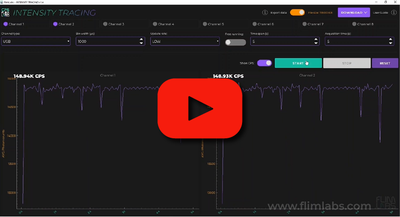
The GUI mode provides advanced functionality for configuring analysis parameters and displaying live-streamed photon data. It allows simultaneous acquisition from up to 8 channels, offering real-time data visualization in the form of plots:

X Axis: represents acquisition time
Y Axis: represents photons intensity

Here an overview of each available feature:

Acquisition channels

The software allows for data acquisition in single-channel or multi-channel mode, with the user able to activate up to 8 channels simultaneously.

For each activated channel, its respective real-time acquisition plot will be displayed on the interface.

The number of active channels affects the size of the exported data file. With the same values set for bin width and acquisition time , the file size grows proportionally to the number of activated channels.

To start acquisition, at least one channel must be activated.

Note: Ensure that the channel activated in the software corresponds to the channel number being used for acquisition on the FLIM LABS Data Acquisition Card.

Connection type

The user can choose the type of connection for data acquisition between SMA and USB connections.

Note: The connection type set in the software must match the actual connection type activated on the FLIM LABS Data Acquisition Card.

Bin width

The user can set a bin width value ranging from 1 to 1,000,000 microseconds (μs). Bin width represents the duration of time to wait for accumulating photon counts in the exported data file. In the interface plots, this value is adjusted to maintain real-time visualization.

The configured bin width value affects the size of the exported data file. With the number of active channels and acquisition time unchanged, the file size grows inversely proportional to the bin width value.

Acquisition mode

Users can choose between two data acquisition modes: free running or fixed acquisition time.

In free running mode, the total acquisition time is not specified. If users deactivate free running mode, they must set a specific acquisition time value.

The chosen acquisition mode impacts the size of the exported data file. Refer to the Export Data section for details.

Acquisition time

When the free running acquisition mode is disabled, users must specify the acquisition time parameter to set the total data acquisition duration. Users can choose a value between 1 and 1800 s (seconds).

For example, if a value of 10 is set, the acquisition will stop after 10 seconds.

The acquisition time value directly affects the final size of the exported data file. Keeping the bin width and active channels values unchanged, the file size increases proportionally to the acquisition time value.

Time span

Time span set the time interval, in seconds, for the last visible data range on the duration x-axis. For instance, if this value is set to 5s, the x-axis will scroll to continuously display the latest 5 seconds of real-time data on the chart. Users can choose a value from 1 to 300 s (seconds).

Show CPS

Users can choose to enable the Show CPS option to display real-time average Photon Count per Second (CPS) in the left-upper corner of active acquisition channel charts. This feature offers an instant insight into signal intensity even when the traces are not actively observed.

CPS threshold

Users can set a numeric value for the Pile-up threshold (CPS) input to highlight it in red with a vibrant effect when the CPS for a specific channel exceeds that threshold.

Export data

Users can choose to export acquired data in .bin file format for further analysis. Refers to this sections for more details:

Parameters table summary

Here a table summary of the configurable parameters:

	data-type	config	default	explanation
`enabled_channels`	number[]	set a list of enabled acquisition data channels (up to 8). e.g. [0,1,2,3,4,5,6,7]	[]	the list of enabled channels for photons data acquisition
`selected_conn_channel`	string	set the selected connection type for acquisition (USB or SMA)	“USB”	If USB is selected, USB firmware is automatically used. If SMA is selected, SMA firmware is automatically used.
`bin_width_micros`	number	Set the numerical value in microseconds. Range: 1-1000000µs	1000 (µs)	the time duration to wait for photons count accumulation.
`free_running_acquisition_time`	boolean	Set the acquisition time mode (True or False)	True	If set to True, the acquisition_time_millis is indeterminate. If set to False, the acquisition_time_millis param is needed (acquisition duration)
`time_span`	number	Time interval, in seconds, for the visible data range on the duration x-axis. Range: 1-300s	5	For instance, if `time_span` is set to 5s, the x-axis will scroll to continuously display the latest 5 seconds of real-time data on the chart
`acquisition_time_millis`	number/None	Set the data acquisition duration. Range: 1-1800s	None	The acquisition duration is indeterminate (None) if free_running_acquisition_time is set to True.
`write_data`	boolean	Set export data option to True/False	False	if set to True, the acquired raw data will be exported locally to the computer
`show_cps`	boolean	Set show cps option to True/False	False	if set to True, user can visualize cps value (average photon count per second) on charts for each active channel
`cps_threshold`	number	Set the CPS threshold	0	If set to a value greater than 0, the user will see the CPS for each channel highlighted in red with a vibrant effect when they exceed the set threshold

Parameters Configuration Saving

Starting from Intensity Tracing v.1.4, the saving of GUI configuration parameters has been automated. Each interaction with the parameters results in the relative value change being stored in a settings.ini internal file.

The configurable parameters which can be stored in the settings file include:

enabled_channels
selected_conn_channel
selected_firmware
bin_width_micros
time_span
acquisition_time_millis
free_running_acquisition_time
write_data
show_cps
cps_threshold

On application restart, the saved configuration is automatically loaded. If the settings.ini file is not found, or a specific parameter has not been configured yet, a default configuration will be set.

Here an example of the settings.ini structure:

[General]
show_cps=true
free_running_mode=false
acquisition_time_millis=100000
bin_width_micros=2000
enabled_channels="[0, 1, 2]"
acquisition_stopped=true
write_data=true
time_span=10
cps_threshold=250000

(back to top)

Long Time Acquisitions and Ring Buffers

The software employs ring buffers to ensure seamless long-time acquisition of photon counts. A ring buffer, also known as a circular buffer, is utilized for efficient handling of cyclic data streams.

A ring buffer is a data structure implemented as a circular array, allowing continuous and cyclic storage of data. It is particularly useful when dealing with repetitive data streams without the need to fill or empty the entire buffer at once. This characteristic makes it well-suited for scenarios requiring constant data access and management.

It’s important to note that, due to the continuous nature of long-time acquisition, the system may consume a significant amount of RAM. In practice, for extended acquisition sessions, we estimate a potential consumption of up to 4 gigabytes of RAM. Users should be mindful of their system’s memory capabilities to ensure smooth operation during extended experiments.

(back to top)

Reader mode

The user can choose to use the software in Reader mode, loading .bin files from external intensity data acquisitions. The user can configure which plots to display, with up to 4 channels shown simultaneously. Additionally, they can view the metadata related to the acquisition and download an image in .png and .eps format that replicates the acquisition graphs.

(back to top)

Console Usage

For a detailed guide about console mode usage follow this link:

Intensity Tracing Console guide

(back to top)

Exported Data Visualization

The application GUI allows the user to export the analysis data in binary file format.

The user can also preview the final file size on the GUI. Since the calculation of the size depends on the values of the parameters enabled_channels, bin_width_micros, free_running_acquisition_time, time_span, and acquisition_time_millis, the value will be displayed if the following actions have been taken:

At least one acquisition channel has been activated (enabled_channels has a length greater than 0).
Values have been set for time_span, acquisition_time_millis, and bin_width_micros.

Here is a code snippet which illustrates the algorithm used for the calculation:

def calc_exported_file_size(app):
    if len(app.enabled_channels) == 0:
        app.bin_file_size_label.setText("")
        return      
    chunk_bytes = 8 + (4 * len(app.enabled_channels))    
    chunk_bytes_in_us =  (1000 * (chunk_bytes * 1000)) / app.bin_width_micros
    if app.free_running_acquisition_time is True or app.acquisition_time_millis is None:
        file_size_bytes = int(chunk_bytes_in_us)
        app.bin_file_size = FormatUtils.format_size(file_size_bytes)
        app.bin_file_size_label.setText("File size: " + str(app.bin_file_size) + "/s")
    else:
        file_size_bytes = int(chunk_bytes_in_us * (app.acquisition_time_millis/1000))
        app.bin_file_size = FormatUtils.format_size(file_size_bytes)
        app.bin_file_size_label.setText("File size: " + str(app.bin_file_size))

For a detailed guide about data export and binary file structure see:

Intensity Tracing Data Export guide

(back to top)

Download Acquired Data

If the Export data option is enabled, the acquisition .bin file and the Python and Matlab scripts for manipulating and displaying the acquired data are automatically downloaded at the end of the acquisition, after the user selects a name for the files.

Note: a requirements.txt file — indicating the dependencies needed to run the Python script - will also be automatically downloaded.

Refer to these sections for more details:

(back to top)

License

Distributed under the MIT License.

(back to top)

Contact

FLIM LABS: info@flimlabs.com

Project Link: FLIM LABS - Intensity Tracing

(back to top)

This site is open source. Improve this page.