spectroscopy-py

Spectroscopy v1.0

Table of Contents

Introduction
GUI Usage
Parameters table summary
Automatic plot update
- Pull from queue function
- Update plot 2 function
Automatic firmware detection
Export Data Visualization
Console usage
Spectroscopy introduction
License
Contact

Introduction

Welcome to FLIM LABS Spectroscopy v1.0 usage guide. In this documentation section, you will find all the necessary information for the proper use of the application’s graphical user interface (GUI). For a general introduction to the aims and technical requirements of the project, read the Spectroscopy Homepage link.

(back to top)

GUI Usage

The GUI mode provides advanced functionality for configuring analysis parameters and displaying live-streamed fluorescence intensity decay data. It allows simultaneous acquisition from up to 8 channels, offering real-time data visualization in the form of plots. There are two types of graphs used to represent the data:

Photon intensity graph:

X Axis: represent aquisition time
Y Axis: represent average photon counts

Photon intensity decay graph:

X Axis: represent aquisition time
Y Axis: represent average photon counts

Here an overview of each available feature:

Sync in and sync out

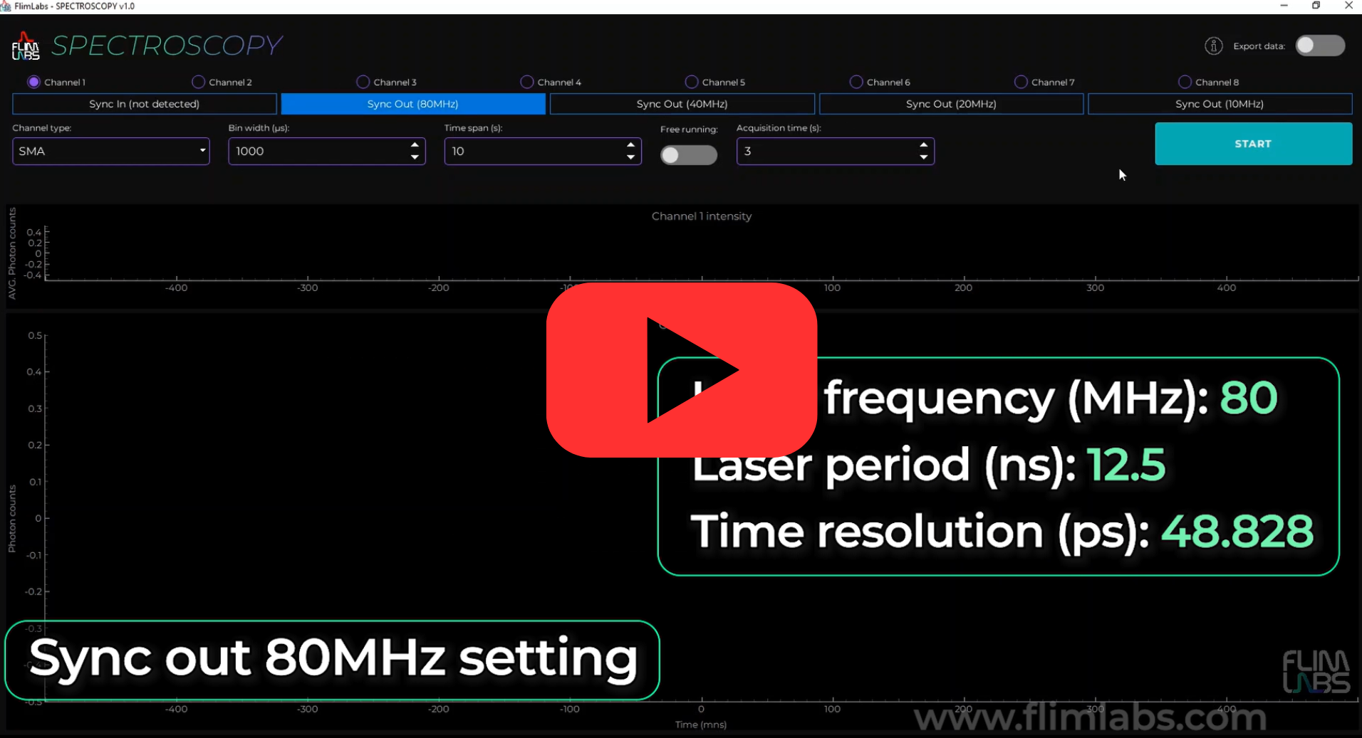
By selecting Sync In, you will automatically initiate the process of measuring your laser’s frequency. Alternatively, by selecting one of the Sync Out options, you can choose the desired frequency (80MHz, 40MHz, 20MHz, 10MHz). When the export data mode is active, the size of the generated file will increase in accordance with the number of active channels.

Selecting the Sync value is essential, as it determines the laser frequency and directly impacts the laser period and the time resolution of the measurements. A higher frequency reduces the laser period, enhancing the time resolution and enabling the capture of events in shorter time intervals.
The X-axis of the graphs reflects the laser period, depicting the time period of a single laser pulse. This aspect is crucial because the decay curve represented on the graph is the sum of curves from each chunk, where each chunk is defined by the bin width refer to the bin width section for more details.

The software automatically adjusts the time resolution according to the selected frequency, ensuring precision.
Each decay curve is represented by 256 points, maintaining this constancy despite changes in frequency or temporal resolution.

Selecting a Sync out of 80MHz, we obtain a laser period of 12.5 ns and a temporal resolution of about 48.828 ps; thus, each point represents an interval of approximately 48.828 ps across the cumulative decay curves.

Conversely, at 20MHz, the laser period extends to 50 ns with a temporal resolution of about 195.312 ps, indicating that each point on the curve corresponds to an interval of approximately 195.312 ps across the cumulative decay curves of each chunk.

Acquisition channels

The software allows for data acquisition in single-channel or multi-channel mode, with the user able to activate up to 8 channels simultaneously.

For each activated channel, its respective real-time acquisition plot will be displayed on the interface.

The number of active channels affects the size of the exported data file. With the same values set for bin width and acquisition time , the file size grows proportionally to the number of activated channels.

To start acquisition, at least one channel must be activated.

Note: Ensure that the channel activated in the software corresponds to the channel number being used for acquisition on the FLIM LABS Data Acquisition Card.

Connection type

The user can choose the type of connection for data acquisition between SMA and USB connections.

Note: The connection type set in the software must match the actual connection type activated on the FLIM LABS Data Acquisition Card.

Bin width

The user can set a bin width value ranging from 100 to 1,000,000 microseconds (μs).

The bin width value specifies the time interval, in microseconds (μs), used to divide the data acquisition into chunks. For each chunk, a theoretical photon decay curve is generated. The final graph represents the cumulative decay curves of each individual chunk. This approach provides a detailed representation of fluorescence over time, illustrating both the intensity and decay of photon signals.

As an example, consider an acquisition time of 10 seconds and a bin width of 10,000 microseconds (μs). This configuration results in the creation of 1000 chunks, each contributing to the overall decay curve displayed in the graph.

This methodology allows users to analyze fluorescence data in a more granular manner, enabling the identification of specific signal characteristics and trends.

The configured bin width value affects the size of the exported data file. With the number of active channels and acquisition time unchanged, the file size grows inversely proportional to the bin width value.

Acquisition mode

Users can choose between two data acquisition modes: free running or fixed acquisition time.

In free running mode, the total acquisition time is not specified. If users deactivate free running mode, they must set a specific acquisition time value.

The chosen acquisition mode impacts the size of the exported data file. Refer to the Export Data section for details.

Acquisition time

When the free running acquisition mode is disabled, users must specify the acquisition time parameter to set the total data acquisition duration. Users can choose a value between 1 and 1800 s (seconds).

For example, if a value of 10 is set, the acquisition will stop after 10 seconds.

The acquisition time value directly affects the final size of the exported data file. Keeping the bin width and active channels values unchanged, the file size increases proportionally to the acquisition time value.

Time span

Time span set the time interval, in seconds, for the last visible data range on the duration x-axis. For instance, if this value is set to 5s, the x-axis will scroll to continuously display the latest 5 seconds of real-time data on the chart. Users can choose a value from 1 to 300 s (seconds).

The time span value, along with update rate affects the maximum number of points maintained on the plot. For further details, refer to the Max Points and Draw Frequency section.

Export data

Users can choose to export acquired data in .bin file format for further analysis. Refers to this sections for more details:

Exported Data Visualization

(back to top)

Parameters table summary

Here a table summary of the configurable parameters:

Parameter	data-type	config	default	explanation
`BIN_WIDTH`	number	Set the numerical value in microseconds	1000	the time duration to wait for photons count accumulation.
`CONNECTION_TYPE`	string	set the selected connection type for acquisition (USB or SMA)	“USB”	If USB is selected, USB firmware is automatically used. If SMA is selected, SMA firmware is automatically used.
`FREE_RUNNING`	boolean	Set the acquisition time mode (True or False)	True	If set to True, the ACQUISITION_TIME is indeterminate. If set to False, the ACQUISITION_TIME param is needed (acquisition duration)
`selected_channels`	number[]	set a list of selected acquisition data channels (up to 8). e.g. [0,1,2,3,4,5,6,7]	[]	the list of selected channels for photons data acquisition
`TIME_SPAN`	number	Time interval, in seconds, for the visible data range on the duration x-axis.	5	For instance, if `time_span` is set to 5s, the x-axis will scroll to continuously display the latest 5 seconds of real-time data on the chart
`ACQUISITION_TIME`	number/None	Set the data acquisition duration	None	The acquisition duration is indeterminate (None) if FREE_RUNNING is set to True.
`sync_out_10_button`	enabled/disabled	Enable or disable the button	False	Choose 10MHz as sync out frequency
`sync_out_20_button`	enabled/disabled	Enable or disable the button	False	Choose 20MHz as sync out frequency
`sync_out_40_button`	enabled/disabled	Enable or disable the button	False	Choose 40MHz as sync out frequency
`sync_out_80_button`	enabled/disabled	Enable or disable the button	True	Choose 80MHz as sync out frequency

(back to top)

Automatic plot update

The software automatically use the pull from queue and update_plots_2 functions in order to update the plots by pulling new data from a queue.

(back to top)

Pull from queue function

The pull_from_a_queue function’s primary objective is to monitor the queue for new data utilizing the Flim Labs API.
Upon detecting new data, the function updates the plots accordingly by calling the update_plot_2 function. If no data is retrieved, the data acquisition process is halted.

def pull_from_queue(self):
        val = flim_labs.pull_from_queue()
        if len(val) > 0:
            for v in val:
                if v == ('end',):  # End of acquisition
                    print("Got end of acquisition, stopping")
                    self.on_start_button_click()
                    self.mode = MODE_STOPPED
                    self.style_start_button()
                    QApplication.processEvents()
                    break
                ((channel,), (time_ns,), intensities) = v
                channel_index = self.selected_channels.index(channel)
                self.update_plots2(channel_index, time_ns, intensities)
                QApplication.processEvents()

(back to top)

Update plot 2 function

The purpose of theupdate_plot_2 function is to update the plots when receiving new datas by the pull_from_queue function.
The function receive three parameters: channel_index, time in nanoseconds time_ns, and a data curve curve.
Then extracts the current x (time) and y (average intensity) data for the specified channel from self.intensity_lines[channel_index].getData().

(back to top)

Update the photon intensity plot

If the current data is undefined or consists solely of a placeholder (for example, if x[0] == 0), it initializes x with the current time converted to seconds (time_ns / 1,000,000,000) and y with the sum of the curve values (np.sum(curve)).
If data already exists, it appends the new data point, converting the time to seconds and calculating the average intensity.

(back to top)

Update the photon intensity decay plot

Extracts the current x (time) and y (photon counts) data for the specified channel from self.decay_curves[channel_index].getData().
Updates the decay curve by adding the current data curve curve to the existing y values, without altering x. This indicates that the curve represents an increment or update of photon counts or intensity for the same time interval already depicted in x.

(back to top)

GUI update

Invokes QApplication.processEvents() to ensure the user interface remains responsive and updates with the new plot data.
Introduces a brief pause (time.sleep(0.01)) to slow down the update process and potentially reduce the load on the UI or the application’s main thread.

def update_plots2(self, channel_index, time_ns, curve):
        x, y = self.intensity_lines[channel_index].getData()
        if x is None or (len(x) == 1 and x[0] == 0):
            x = np.array([time_ns / 1_000_000_000])
            y = np.array([np.sum(curve)])
        else:
            x = np.append(x, time_ns / 1_000_000_000)
            y = np.append(y, np.sum(curve))

        self.intensity_lines[channel_index].setData(x, y)
        x, y = self.decay_curves[channel_index].getData()
        self.decay_curves[channel_index].setData(x, curve + y)
        QApplication.processEvents()
        time.sleep(0.01)

(back to top)

Automatic firmware detection

In order to start the acquisition process, the function begin_spectroscopy_experiment automatically detect the firmware version of your FLIM LABS acquisition card.

(back to top)

Exported Data Visualization

The application GUI allows the user to export the analysis data in binary file format.

The user can also preview the final file size on the GUI. Since the calculation of the size depends on the values of the parameters SETTINGS_FREE_RUNNING, SETTINGS_ACQUISITION_TIME, SETTINGS_BIN_WIDTH and selected_channels, the value will be displayed if the following actions have been taken:

At least one acquisition channel has been activated (selected_channels has a length greater than 0).
export_data_control is active

Here is a code snippet which illustrates the algorithm used for the calculation:

def calc_exported_file_size(self):
        free_running = self.settings.value(SETTINGS_FREE_RUNNING, DEFAULT_FREE_RUNNING)
        acquisition_time = self.settings.value(SETTINGS_ACQUISITION_TIME, DEFAULT_ACQUISITION_TIME)
        bin_width = self.settings.value(SETTINGS_BIN_WIDTH, DEFAULT_BIN_WIDTH)

        if free_running is True or acquisition_time is None:
            file_size_MB = len(self.selected_channels) * (1000 / int(bin_width))
            self.bin_file_size = format_size(file_size_MB * 1024 * 1024)
            self.bin_file_size_label.setText("File size: " + str(self.bin_file_size) + "/s")
        else:
            file_size_MB = int(acquisition_time) * len(self.selected_channels) * (1000 / int(bin_width))
            self.bin_file_size = format_size(file_size_MB * 1024 * 1024)
            self.bin_file_size_label.setText("File size: " + str(self.bin_file_size))

(back to top)

Console Usage

For a detailed guide about console mode usage follow this link:

Spectroscopy Console guide

(back to top)

Spectroscopy introduction

Check the spectroscopy introduction documentation at these link:

Spectroscopy introduction

License

Distributed under the MIT License.

(back to top)

Contact

FLIM LABS: info@flimlabs.com

Project Link: FLIM LABS - Spectroscopy

(back to top)